  1
  2
  3
  4
  5
  6
  7
  8
  9
 10
 11
 12
 13
 14
 15
 16
 17
 18
 19
 20
 21
 22
 23
 24
 25
 26
 27
 28
 29
 30
 31
 32
 33
 34
 35
 36
 37
 38
 39
 40
 41
 42
 43
 44
 45
 46
 47
 48
 49
 50
 51
 52
 53
 54
 55
 56
 57
 58
 59
 60
 61
 62
 63
 64
 65
 66
 67
 68
 69
 70
 71
 72
 73
 74
 75
 76
 77
 78
 79
 80
 81
 82
 83
 84
 85
 86
 87
 88
 89
 90
 91
 92
 93
 94
 95
 96
 97
 98
 99
100
101
102
103
104
105
106
107
108
109
110
111
112
113
114
115
| from sklearn.model_selection import train_test_split
from sklearn.metrics import accuracy_score、
import matplotlib.pyplot as plt
from keras import regularizers
from sklearn.preprocessing import MinMaxScaler
from keras.models import Sequential
from keras.layers import Dense, Dropout
from sklearn import preprocessing
def NN_Plot(i, X, Y, model_output = False):
# i 为需要输出图表的y轴标签;
# X 为自变量的数据集;
# Y 为输出变量的数据;
# model_output 表示是否返回 训练后的模型;
# 1. 数据集标准化
min_max_scaler = preprocessing.MinMaxScaler()
X_scale = min_max_scaler.fit_transform(X)
# 2.训练集和验证集的划分
X_train, X_test, Y_train, Y_test = train_test_split(X_scale, Y, test_size=0.3, random_state = n)
# 3. 模型的结构设计
model = Sequential() # 初始化,很重要
model.add(Dense(units = 1000, # 输出大小,也是该层神经元的个数
activation='relu', # 激励函数-RELU
input_shape=(X_train.shape[1],) # 输入大小, 也就是列的大小
))
model.add(Dropout(0.3)) # 丢弃神经元链接概率
model.add(Dense(units = 1000,
kernel_regularizer=regularizers.l2(0.01), # 施加在权重上的正则项
activity_regularizer=regularizers.l1(0.01), # 施加在输出上的正则项
activation='relu' # 激励函数
# bias_regularizer=keras.regularizers.l1_l2(0.01) # 施加在偏置向量上的正则项
))
model.add(Dropout(0.15))
model.add(Dense(units = 500,
kernel_regularizer=regularizers.l2(0.01), # 施加在权重上的正则项
activity_regularizer=regularizers.l1(0.01), # 施加在输出上的正则项
activation='relu' # 激励函数
# bias_regularizer=keras.regularizers.l1_l2(0.01) # 施加在偏置向量上的正则项
))
model.add(Dropout(0.15))
model.add(Dense(units = 500,
kernel_regularizer=regularizers.l2(0.01), # 施加在权重上的正则项
activity_regularizer=regularizers.l1(0.01), # 施加在输出上的正则项
activation='relu' # 激励函数
# bias_regularizer=keras.regularizers.l1_l2(0.01) # 施加在偏置向量上的正则项
))
model.add(Dropout(0.2))
model.add(Dense(units = 1,
activation='linear',
kernel_regularizer=regularizers.l2(0.01) # 线性激励函数回归一般在输出层用这个激励函数
))
model.compile(optimizer='adam',
loss='mse', # 损失函数为均方误差
metrics=['accuracy'])
# 4. 模型的训练,可以自行修改batch——size大小和epoch大小
hist = model.fit(X_train, Y_train,
batch_size = 32, epochs=250, verbose = 2,
validation_data=(X_test, Y_test))
# 5. 模型的损失值变化图绘制
plt.plot(hist.history['loss'])
plt.plot(hist.history['val_loss'])
plt.title('Model loss')
plt.ylabel('Loss')
plt.xlabel('Epoch')
plt.legend(['Train', 'Val'], loc='upper right')
plt.show()
y_pred = model.predict(X_test)
y_pred_train = model.predict(X_train)
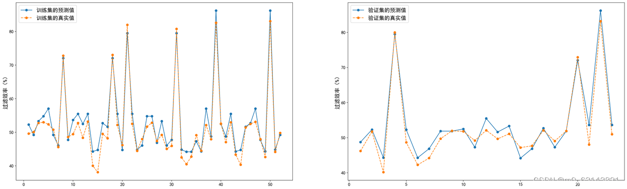
# 6. 模型在训练集和测试集上的拟合程度图绘制
plt.figure(figsize=(30,9),dpi = 200)
plt.subplot(1,2,1)
ls_x_train = [x for x in range(1, len(y_pred_train.tolist())+1)]
plt.plot(ls_x_train, y_pred_train.tolist(), label = '训练集的预测值' , marker = 'o')
plt.plot(ls_x_train, Y_train.iloc[:,0].tolist(), label = '训练集的真实值',linestyle='--', marker = 'o' )
plt.ylabel(i, fontsize = 15)
plt.legend(fontsize = 15)
plt.xticks(fontsize = 12)
plt.yticks(fontsize = 12)
plt.subplot(1,2,2)
ls_x = [x for x in range(1, len(y_pred.tolist())+1)]
plt.plot(ls_x, y_pred.tolist(), label = '验证集的预测值' , marker = 'o')
plt.plot(ls_x, Y_test.iloc[:,0].tolist(), label = '验证集的真实值',linestyle='--',marker = 'o')
plt.ylabel(i, fontsize = 15)
plt.xticks(fontsize = 12)
plt.yticks(fontsize = 12)
plt.legend(fontsize = 15)
# R方的计算
r2_train = R_2(Y_train.iloc[:,0].tolist(), y_pred_train)
r2_test = R_2(Y_test.iloc[:,0].tolist(), y_pred)
print([r2_train, r2_test, (r2_train+r2_test)/2 ])
# 是否返回训练得到的模型
if model_output==True:
return [model, min_max_scaler]
def R_2(y, y_pred):
y_mean = mean(y)
sst = sum([(x-y_mean)**2 for x in y])
ssr = sum([(x-y_mean)**2 for x in y_pred])
sse = sum([(x-y)**2 for x,y in zip(y_pred, y)])
return 1-sse/sst
|